Image Features

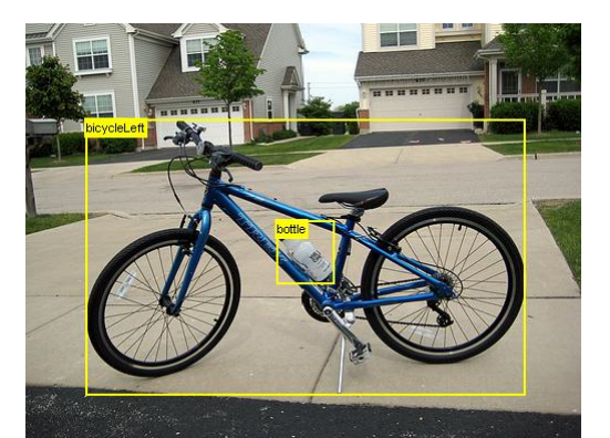
• Image features are essentially vectors that are a compact representation of images •
• They represent important information shown in an image •
• Intuitive examples of image features:
  • Blobs –
  • Edges –
  • Corners –
  • Ridges –
  • Circles –
  • Ellipses –
  • Lines –
  • Etc…

We need to represent images as feature vectors for further processing in a more efficient and robust way

Examples of further processing include: –

• Object detection –
• Image segmentation –
• Image classification –
• Content-based image retrieval –
• Image stitching –
• Object tracking

Properties of Features

• Why not just use pixels values directly? –
  • Pixel values change with light intensity, colour and direction – They also change with camera orientation – And they are highly redundant • Repeatability (robustness) – Should be detectable at the same locations in different images despite changes in illumination and viewpoint • Saliency (descriptiveness) – Similar salient points in different images should have similar features • Compactness (efficiency) – Fewer features – Smaller features

Image Pre-processing

Feature Representation

Pattern Recognition

Post-processing

Feature Types

• Colour features –
  • Colour histogram –
  • Colour moments •
• Texture features –
  • Haralick texture features –
  • Local binary patterns (LBP) – Scale-invariant feature transform (SIFT) –
  • Texture feature encoding •
• Shape features –
  • Basic shape features –
  • Shape context –
  • Histogram of oriented gradients (HOG)

Colour Features

Colour is the simplest feature to compute, and is invariant to image scaling, translation and rotation • Example: colour-based image retrieval

Colour Histogram

Represent the global distribution of pixel colours in an image – Step 1: Construct a histogram for each colour channel (R, G, B) – Step 2: Concatenate the histograms (vectors) of all channels as the final feature vector

Colour Moments

Application Example

Texture Features

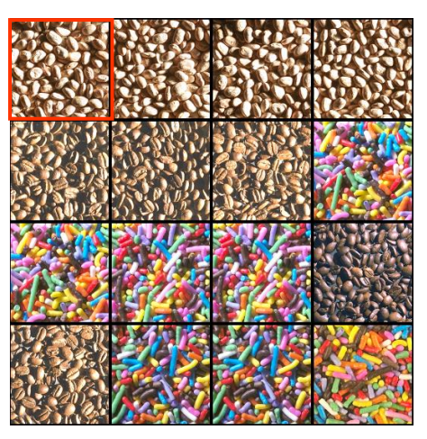
• Texture is a powerful discriminating feature for identifying visual patterns with properties of homogeneity that cannot result from the presence of only a single color or intensity •
• Example: texture classification

Haralick Features

• Haralick features give an array of statistical descriptors of image patterns to capture the spatial relationship between neighbouring pixels, that is, textures –
  • Step 1: Construct the gray-level co-occurrence matrix (GLCM) –
  • Step 2: Compute the Haralick feature descriptors from the GLCM

• Step 1: Construct the GLCMs –
  • Given a distance d at an orientation angle θ – Compute the co-occurrence count (or probability) of going from a gray level l 1 to another gray level l 2 with an intersample spacing of d along the axis making an angle θ with the x axis and denote this as p(d, θ)(l 1, l 2) – Construct the matrix P(d, θ) with the elements (l 1, l 2) being p(d, θ)(l 1, l 2) – If the number of distinct gray levels in the quantized image is L, then the cooccurrence matrix P will be of size L×L

For computational efficiency, the number of gray levels (L) can be reduced by binning (similar to histogram binning), e.g. L = 256/n, with n a constant factor. – Different co-occurrence matrices can be constructed by using various combinations of distance (d) and angular directions (θ). – On their own, these co-occurrence matrices do not provide any measure of texture that can easily be used as texture descriptors. – The information in the co-occurrence matrices needs to be further extracted as a set of feature values => Haralick descriptors.

Application Example

Scale-Invariant Feature Transform

• SIFT feature describes the texture features in a localised region around a keypoint
• SIFT descriptor is invariant to uniform scaling, orientation, and partially invariant to affine distortion and illumination changes
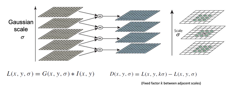
  • Scale-Space Extrema Detection： Find maxima/minima in DoG（Difference of Gaussian） images across scales
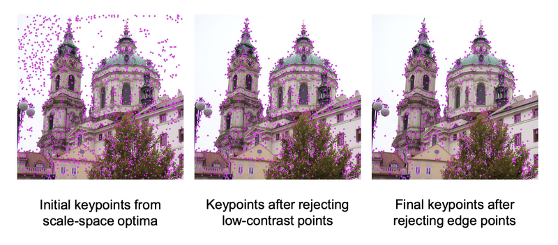
  • Keypoint Localization：Discarding low-contrast keypoints Eliminating edge responses
  • Orientation Assignment：Achieve rotation invariance
  • Keypoint Descriptor：Compute gradient orientation histograms

SIFT Extrema Detection

Detect maxima and minima in the scale space of the image

SIFT Keypoint Localization

• Improve and reduce the set of found keypoints
  • Use 3D quadratic fitting in scale-space to get subpixel optima –
  • Reject low-contrast and edge points using Hessian analysis
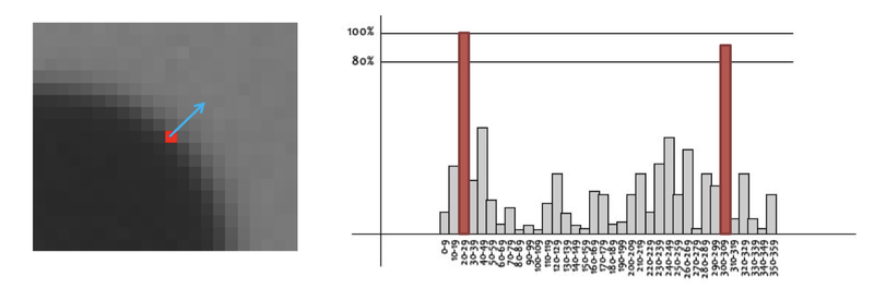
• Estimate keypoint orientation using local gradient vectors – Make an orientation histogram of local gradient vectors – Find the dominant orientation from the main peak of the histogram – Create additional keypoint for second highest peak if >80%

SIFT Orientation Assignment

• Estimate keypoint orientation using local gradient vectors
  • Make an orientation histogram of local gradient vectors
  • Find the dominant orientation from the main peak of the histogram
  • Create additional keypoint for second highest peak if >80%

SIFT Keypoint Descriptor

• 4 x 4 array of gradient histogram weighted by magnitude
• 8 bins in gradient orientation histogram
• Total 8 x 4 x 4 array = 128 dimensions
• 4 x 4 array of gradient histogram weighted by magnitu de

Descriptor Matching

Image stitching – Find SIFT keypoints and feature correspondences

Fitting and Alignment

Given matched points A and B, estimate the transformation Example for translation:

Feature Encoding

Global encoding of local SIFT features – Integrate the local features (SIFT keypoint descriptors) of an image into a global vector to represent the whole image

Most popular method: Bag-of-Words (BoW) – The variable number of local image features are encoded into a fixed-dimensional histogram to represent each image

• Bag-of-Words (BoW) – step 1 – Create the vocabulary from the set of local descriptors (SIFT keypoint descriptors) extracted from the training data – This vocabulary represents the categories of local descripto